Show code cell source Hide code cell source

import ase
import matplotlib.pyplot as plt
import numpy as np
import xarray
from abtem.bloch import StructureFactor
from tqdm.auto import tqdm

import abtem

xarray.set_options(display_expand_data=False)

<xarray.core.options.set_options at 0x2064f5c5a50>

Convergence

In this tutorial, we go through how to ensure a multislice simulation with respect to three major convergence parameters: real space sampling, slice thickness and the size of the ensemble, when calculating ensemble means.

We start by setting the precission to 64-bit floating point, the default is 32-bit, as calculations with extremely small samplings and slice thicknesses can lead to overflow.

abtem.config.set({"precision": "float64"})

<abtem.core.config.set at 0x2064f486010>

Slice thickness

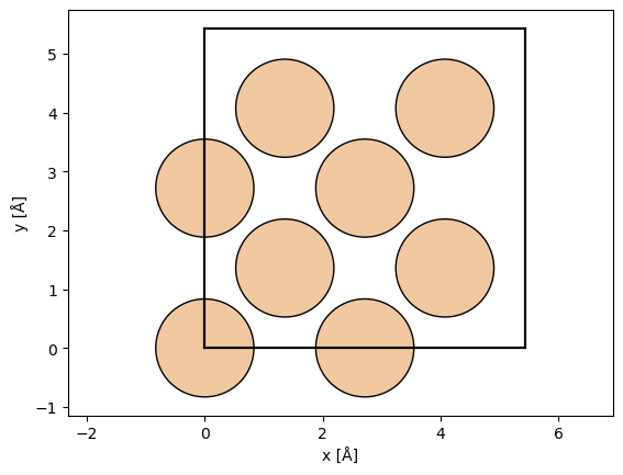
We now turn convergence with respect to slice thickness, our test system is a simulation diffraction patterns with an acceleration voltage of \(200 \ \mathrm{keV}\) and a real space sampling of \(0.02 \ \mathrm{Å}\).

atoms = ase.build.bulk("Si", cubic=True)
abtem.show_atoms(atoms)

wave = abtem.PlaneWave(energy=100e3, sampling=0.02)

We use a geometric sequence halving the slice thickness at each step, starting from the thickness of the entire unit cell, \(a/1, a/2, a/4, ..., a/256\).

thickness_fractions = np.array([2**n for n in np.arange(0, 9)])

thicknesses = atoms.cell[2, 2] / thickness_fractions

thicknesses

array([5.43      , 2.715     , 1.3575    , 0.67875   , 0.339375  ,
       0.1696875 , 0.08484375, 0.04242187, 0.02121094])

We test both finite and infinite potential integrals, below the calculations are set up.

# Initialize a dictionary to store exit wave data for different projections.
exit_waves_lists = {"finite": [], "infinite": []}

# Loop through specified slice thicknesses and projections.
for thickness in thicknesses:
    for projection in exit_waves_lists:

        # Create a potential for the given projection and thickness.
        potential_unit = abtem.Potential(
            atoms,
            projection=projection,
            slice_thickness=thickness,
            sampling=wave.sampling,
        )

        # Define a crystal potential with the potential unit repeated in the z-direction.
        potential = abtem.CrystalPotential(potential_unit, repetitions=(1, 1, 6))

        # Calculate the exit wave using the multislice method.
        exit_wave = wave.multislice(potential)

        # Append the exit wave to the corresponding list in the dictionary.
        exit_waves_lists[projection].append(exit_wave)

We stack all the results to allow for parallelization and to make further analysis easier.

# Define an OrdinalAxis object to represent metadata for the axis.
axes_metadata = abtem.core.axes.OrdinalAxis(
    label="slice thickness", values=[f"a/{f}" for f in thickness_fractions]
)

# Stack the finite exit waves along a new axis using the defined axes metadata.
stacks = [
    abtem.stack(value, axis_metadata=axes_metadata)
    for value in exit_waves_lists.values()
]

# Define new axes metadata, now labeling the axis as "projection"
axes_metadata = abtem.core.axes.OrdinalAxis(
    label="projection", values=list(exit_waves_lists.keys())
)

# Stack the finite and infinite exit waves along a new 'projection' axis.
exit_waves = abtem.stack(
    stacks,  # List of the two exit wave stacks to combine
    axis_metadata=axes_metadata,  # The new axis metadata
)

# Swap the first and second axes of the exit_waves array for plotting
exit_waves = abtem.array.swapaxes(exit_waves, 0, 1)

exit_waves.axes_metadata

type           label            coordinates
-------------  ---------------  ------------------
OrdinalAxis    slice thickness  -
OrdinalAxis    projection       -
RealSpaceAxis  x [Å]            0.00 0.02 ... 5.41
RealSpaceAxis  y [Å]            0.00 0.02 ... 5.41

Compute all the calculations.

exit_waves.compute()

[########################################] | 100% Completed | 95.83 ss

<abtem.waves.Waves at 0x2064f7f3050>

We show the exit waves up to a slice thickness of \(a/16\), as it becomes difficult to tell differences by eye after this point.

exit_waves[:5].show(explode=True, common_color_scale=True, figsize=(12, 6));

To make the comparison quantitative, we obtain the diffraction spots. We convert the abTEM object to an Xarray DataArray to use its more powerful generic data manipulation tools, the abTEM AxisMetadata is converted to coordinates.

spots = (
    exit_waves.diffraction_patterns()
    .crop(140)
    .to_cpu()
    .index_diffraction_spots(atoms.cell, centering="F")
)

spots = spots**0.5

data = spots.to_data_array()

data

<xarray.DataArray (slice thickness: 9, projection: 2, hkl: 529)> Size: 76kB
0.9431 2.285e-08 0.07718 2.15e-09 ... 0.002454 0.00113 0.002416 0.0004934
Coordinates:
  * slice thickness  (slice thickness) <U5 180B 'a/1' 'a/2' ... 'a/128' 'a/256'
  * projection       (projection) <U8 64B 'finite' 'infinite'
  * hkl              (hkl) <U10 21kB '0 0 0' '0 2 0' ... '-1 -11 -1' '-1 -9 -1'
Attributes:
    long_name:  intensity
    units:      arb. unit

xarray.DataArray

• slice thickness: 9
• projection: 2
• hkl: 529

• 0.9431 2.285e-08 0.07718 2.15e-09 ... 0.00113 0.002416 0.0004934

  array([[[9.43148698e-01, 2.28453379e-08, 7.71812990e-02, ...,
           8.08962998e-10, 1.41260287e-09, 2.33455793e-09],
          [9.42886968e-01, 6.70010037e-17, 7.72354908e-02, ...,
           2.01827223e-18, 8.24251295e-19, 6.15122013e-19]],
  
         [[9.43016889e-01, 1.44529021e-03, 7.78756606e-02, ...,
           1.29695257e-03, 1.26662373e-03, 1.14881665e-03],
          [9.42924481e-01, 7.00190879e-17, 7.69361085e-02, ...,
           7.28775018e-18, 2.53800204e-03, 4.67825207e-18]],
  
         [[9.42720979e-01, 1.60101173e-04, 7.84523505e-02, ...,
           1.34440904e-03, 1.31314697e-03, 1.24589830e-03],
          [9.42890695e-01, 2.19824824e-03, 7.68083704e-02, ...,
           1.12995039e-03, 2.41609209e-03, 4.93423905e-04]],
  
         ...,
  
         [[9.42942531e-01, 2.87047102e-04, 7.71298292e-02, ...,
           1.64665466e-03, 1.41975018e-03, 1.34699996e-03],
          [9.42890760e-01, 2.19824735e-03, 7.68082495e-02, ...,
           1.12995234e-03, 2.41608155e-03, 4.93421056e-04]],
  
         [[9.42961676e-01, 2.88060647e-04, 7.70967307e-02, ...,
           1.64682508e-03, 1.41848549e-03, 1.34824797e-03],
          [9.42890820e-01, 2.19824630e-03, 7.68082204e-02, ...,
           1.12995151e-03, 2.41608392e-03, 4.93420162e-04]],
  
         [[9.42963888e-01, 2.88301604e-04, 7.70922430e-02, ...,
           1.64723024e-03, 1.41840548e-03, 1.34875802e-03],
          [9.42890860e-01, 2.19824626e-03, 7.68082097e-02, ...,
           1.12995120e-03, 2.41608594e-03, 4.93419260e-04]]])

• Coordinates: (3)
  • slice thickness
    (slice thickness)
    <U5
    'a/1' 'a/2' ... 'a/128' 'a/256'

    array(['a/1', 'a/2', 'a/4', 'a/8', 'a/16', 'a/32', 'a/64', 'a/128', 'a/256'],
          dtype='<U5')

  • projection
    (projection)
    <U8
    'finite' 'infinite'

    array(['finite', 'infinite'], dtype='<U8')

  • hkl
    (hkl)
    <U10
    '0 0 0' '0 2 0' ... '-1 -9 -1'

    array(['0 0 0', '0 2 0', '0 4 0', ..., '-1 -13 -1', '-1 -11 -1', '-1 -9 -1'],
          dtype='<U10')

• Indexes: (3)
  • slice thickness
    PandasIndex

    PandasIndex(Index(['a/1', 'a/2', 'a/4', 'a/8', 'a/16', 'a/32', 'a/64', 'a/128', 'a/256'], dtype='object', name='slice thickness'))

  • projection
    PandasIndex

    PandasIndex(Index(['finite', 'infinite'], dtype='object', name='projection'))

  • hkl
    PandasIndex

    PandasIndex(Index(['0 0 0', '0 2 0', '0 4 0', '0 6 0', '0 8 0', '0 10 0', '0 12 0',
           '0 14 0', '0 20 -2', '0 -20 -2',
           ...
           '-1 13 -1', '-1 15 -1', '-1 17 -1', '-1 19 -1', '-1 -19 -1',
           '-1 -17 -1', '-1 -15 -1', '-1 -13 -1', '-1 -11 -1', '-1 -9 -1'],
          dtype='object', name='hkl', length=529))

• Attributes: (2)

  long_name :

  intensity

  units :

  arb. unit

spots[:5].show(explode=True, figsize=(12, 6), scale=0.05, annotations=False)

<abtem.visualize.visualizations.Visualization at 0x2060082e810>

To calculate an error we need to choose a reference calculation, here we use the calculation with the finest finite projection integrals.

# Select the reference data point
reference = data.sel({"projection": "finite", "slice thickness": "a/256"})

# Calculate the difference between each data point in 'data' and the selected reference.
difference = data - reference

# Define a list of Miller indices to plot
miller_indices = [
    "0 0 0",
    "2 -2 0",
    "4 0 0",
]

# Create a 1-row, 3-column subplot structure and set the figure size.
fig, axes = plt.subplots(1, 3, figsize=(12.5, 4))

# Loop through each subplot axis and corresponding Miller index.
for ax, miller_index in zip(axes, miller_indices):
    # Plot the line graph of the difference data selected by Miller index,
    # with different lines for each projection.
    difference.sel(hkl=miller_index).plot.line(hue="projection", ax=ax)

    # Add a horizontal line at y=0 for reference
    ax.axhline(0, color="gray", linestyle="--")
    ax.ticklabel_format(axis='y', scilimits=[-3, 3])

plt.tight_layout()

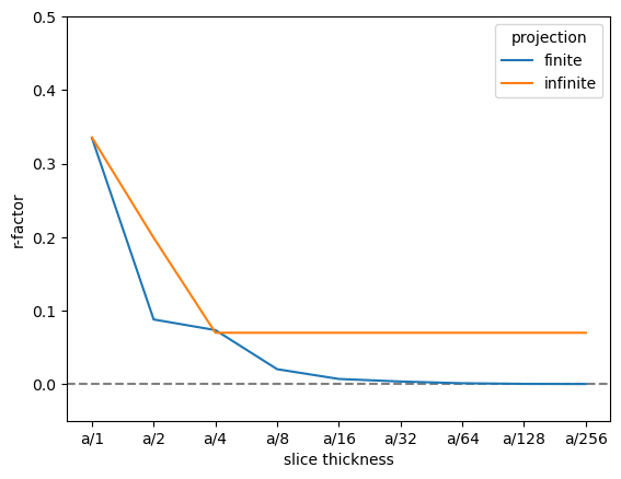
As there are four atomic planes in the unit cell, any smaller slice thickness beyond \(a/4\) does not improve the accuracy, when using the infinite projection. Actually, a any slice thickness that does not have \(4\) as a factor may be slightly worse, since such a slice thickness requires shifting the atoms along \(z\).

Here, we use the R-factor, which in crystallogrphy is a measure of the difference between the observed (\(F_{obs}\)) and calculated (\(F_{calc}\)) structure factor amplitudes in crystallography. $\( R = \frac{\sum |F_{\text{obs}} - F_{\text{calc}}|}{\sum |F_{\text{obs}}|} \)$

is a measure of the difference between the observed () and calculated () structure factor amplitudes in crystallography. The R-factor is used to assess the quality of a crystal structure model.

We find that the R-factor is converged to within \(1 \%\) for a slice thickness of \(a/16\), as stated above the infinite projection cannot improve beyound the the atomic planes, hence

r_factor = np.abs(data - reference).sum("hkl") / np.abs(data).sum("hkl")

fig, ax = plt.subplots()
ax.axhline(0, color="gray", linestyle="--")
r_factor.plot.line(hue="projection", ax=ax)

ax.set_ylabel("r-factor")
ax.set_ylim([-0.05, 0.5]);