Show code cell source Hide code cell source

import ase
import numpy as np

import abtem

Customizing abTEM

In this tutorial, we describe how to extend abTEM and introduce a few general concepts on how the library works. This tutorial requires familarity with NumPy and in some parts a basic understanding of Dask.

Currently Under Construction

This section uses a new relatively untested feature.

The ArrayObject

In abTEM we describe the \(xy\)-part of a wave function on a 2D grid using a 2D NumPy (or CuPy) array, an ensemble of such wave functions may also be described as a single array with an additional dimensions for each ensemble dimension, for example multiple different positions. We encapsulate that array together with metadata such as the energy and real-space extent and call it a Waves object.

The Waves are an example of an ArrayObject which is the base class for any object in abTEM represented mainly by a single NumPy (or CuPy) array and some metadata for example the energy and sampling of the wave function, another example is the PotentialArray. All ArrayObjects may also be be lazy utilizing a Dask array.

Objects such as the Probe and Potential are not ArrayObject’s, they act as an interface to create Waves and PotentialArray.

atoms = ase.build.mx2("WS2", vacuum=2)
atoms = abtem.orthogonalize_cell(atoms) * (7, 4, 1)

potential = abtem.Potential(atoms, sampling=0.05)

probe = abtem.Probe(energy=120e3, semiangle_cutoff=30)

probe.grid.match(potential)

waves = probe.build()

However, we can run the .build method to create Waves.

waves = probe.build()

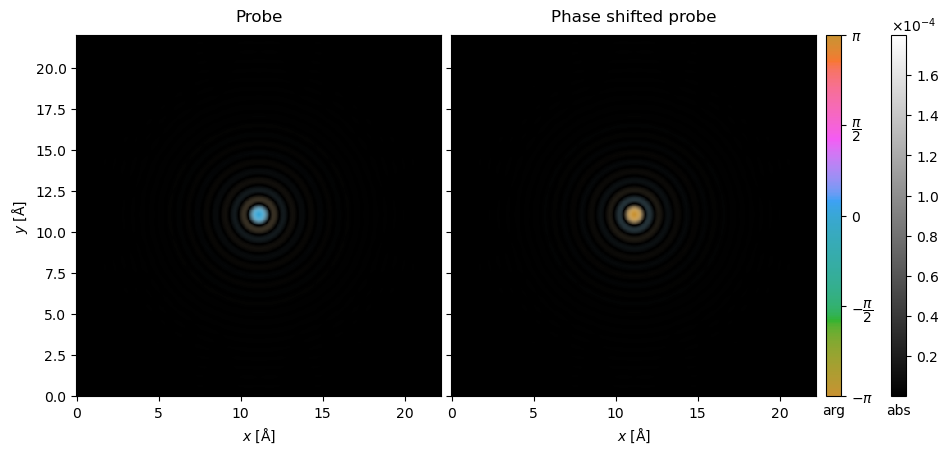
You can create any custom wave function by creating a Waves object from a NumPy array. For example, we can take the array created by the Probe and apply a phase shift.

array = waves.array.compute()  # compute makes the Dask array into a NumPy array

new_array = array * np.exp(-1.0j * np.pi)

Any 2D Numpy array can be used to create a custom Waves object. To fully define a Waves object you also need to at least provide the energy and sampling.

custom_waves = abtem.Waves(
    array=new_array, energy=waves.energy, sampling=waves.sampling
)

To utilize Dask, we can use the .lazy method.

custom_waves = custom_waves.lazy()

custom_waves.array

Array Chunk Bytes 1.50 MiB 1.50 MiB Shape (446, 441) (446, 441) Dask graph 1 chunks in 1 graph layer Data type complex64 numpy.ndarray

stack = abtem.stack((waves, custom_waves), ("Probe", "Phase shifted probe"))

stack = stack.compute().to_images(convert_complex=False)

[########################################] | 100% Completed | 102.92 ms

stack.show(
    explode=True, cbar=True, common_color_scale=True, figsize=(10, 10)
);

Lazy function application

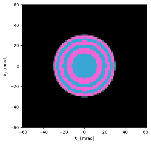
Next we will apply a somewhat more complicated function to the wave function array, a patterned phase plate as for example used in MIDI-STEM. The function below takes a Waves object and a set of angles for where the phase should be flipped by \(\pi / 2\). The function uses mostly standard NumPy apart from some utility functions from abTEM.

We get the spatial frequencies and wavelength from the Waves object.

We use the get_array_module function to make our code agnostic to the array module. This function will return either the NumPy or the CuPy module, depending on the array type, thus enabling the relevant code to work on GPU’s.

We import fft2_convolve from abTEM, this function calculates the FFT convolution using the library provided in the config FFTW, MKL or NumPy on CPU and cuFTT on GPU.

from abtem.core.backend import get_array_module
from abtem.core.fft import fft2_convolve


def phase_flip(
    waves: abtem.Waves,
    max_angle: float,
    num_flips: int,
    power: float,
    phase_shift: float = np.pi / 2,
) -> np.array:
    """
    Applies a radial phase flipping in reciprocal space to the input wave function array.

    Parameters
    ----------
    waves : Waves
        The abTEM electron wavefunction object.
    max_angle : float
        The maximum angle used to normalize the radial frequency at which phase flipping occurs [mrad].
    num_flips : int
        The number of flips in the phase applied within max_angle.
    power : float
        The exponent used in the power law scaling of frequency of phase flipping with radial spatial frequency.
    phase_shift : float, optional
        The phase shift value in radians applied to the flipped regions. Defaults to pi / 2.

    Returns
    -------
    np.ndarray
        An array representing the convolved wavefunction after the phase flip has been applied.
    """

    # Get spatial frequencies for the wave grid.
    kx, ky = waves.grid.spatial_frequencies()

    # Calculate the square of radial frequencies.
    k = np.sqrt(kx[:, None] ** 2 + ky[None] ** 2)

    # Convert max_angle to spatial frequencies, adjusted
    max_k = max_angle / waves.wavelength / 1e3

    # Apply power scaling to the radial frequencies and normalize.
    k_normed = (k / max_k) ** power

    # Generate a phase flip map using a sinusoidal function of the normalized radial frequencies,
    # where the sign of the sine function determines the flip condition.
    phase_flip_map = np.sin(k_normed * np.pi * (num_flips + 1)) < 0

    # We make our code device agnostic.
    xp = get_array_module(waves.array)
    phase_flip_map = xp.asarray(phase_flip_map)

    # Create a phase shift array for flipping by pi/2 radians.
    phase_shift = xp.exp(1.0j * phase_shift * phase_flip_map)

    # Convolve wave array with phase shift in Fourier space.
    array = fft2_convolve(waves.array, phase_shift)

    return array

We build a Waves object and apply the phase_flip function.

# We make sure to build the probe at (0., 0.) instead of the default center
waves = probe.build((0.0, 0.0))

waves.array = phase_flip(waves, max_angle=30.0, num_flips=5, power=2.0)

diffraction = waves.diffraction_patterns(return_complex=True).crop(80).compute()

[########################################] | 100% Completed | 203.23 ms

diffraction.show(cmap="hsluv");

The phase_flip function is applied lazily to the waves.

waves.is_lazy

True

There is a subtle issue here. The phase_flip_map array is calculated at the point of call, this is fine in this case, but goes against the idea of lazy evaluation. In addition the phase_flip_map array has to be placed into the Dask task graph, which can result in expensive serialization for distributed calculations.

The issue is quite simply overcome by using the apply_func method, which will apply the phase_flip function lazily when the Waves are lazy. In addition, waves.array inside the function is non-lazy at the point of compute and only the angles array is embedded in the task graph.

waves = probe.build((0.0, 0.0))

waves = waves.apply_func(phase_flip, max_angle=30.0, num_flips=5, power=2.0)

The scan method can be used as usual.

Note

The scan objects shifts the Waves based on \((x,y)=(0,0)\). So, make sure the probe wave function is placed at (0, 0) before applying a scan. It also bears noting that resolving properties such as the scan Nyquist sampling based on a Waves object may fail.

scan = abtem.GridScan(
    start=(0, 0),
    end=(1 / 7, 1 / 4),
    sampling=0.4,
    fractional=True,
    potential=atoms,
)

waves = probe.build(scan=(0.0, 0.0)).apply_func(
    phase_flip, max_angle=30, num_flips=5, power=2
)

scanned_waves = waves.scan(scan=scan, potential=potential)

diffraction_patterns = scanned_waves.diffraction_patterns(return_complex=True)

diffraction_patterns.compute()

[########################################] | 100% Completed | 7.38 sms

<abtem.measurements.DiffractionPatterns at 0x1a0c8599610>

We show the result as an exploded plot.

diffraction_patterns[:5, 0].crop(60).show(explode=True, figsize=(10, 6));

Object-oriented implementation (WavesTranform)

A more formal extension to abTEM may be accomplished by subclassing the WavesTransform or its parent class ArrayObjectTransform. By extending abTEM this way, the implementation follows the object-oriented design of the code. For simulations with a large number of tasks this implementation may also allow abTEM to better optimize the Dask task graph by merging tasks.

In this section, we show how to implement the example from the preceding section using a WavesTransform. We will create a new PhaseRamp object that takes the argument gradient, to do this we need three things:

• Implement the private _calculate_new_array method. This method takes a Waves object and returns a NumPy array of the same shape (unless otherwise specified, see further on)

• All input arguments should be exposed as public properties

• Add docstrings using the NumPy docstring format

from typing import Sequence


class PatternedPhasePlate(abtem.transform.WavesTransform):
    """
    A patterned phase plate modifying the phase of an electron wavefunction at specific angles.

    Parameters
    ----------
    angles: sequence of float
        A sequence of angles at which the phase plate will flip the phase of the electron wavefunction [mrad].
    """

    def __init__(self, max_angle, num_flips, power):
        self.max_angle = max_angle
        self.num_flips = num_flips
        self.power = power
        super().__init__()

    def _calculate_new_array(self, waves: abtem.Waves) -> np.ndarray:
        return phase_flip(waves, self.max_angle, self.num_flips, self.power)

We can apply our PatternedPhasePlate object using the apply_transform method, which in addition to

phase_plate = PatternedPhasePlate(30, 5, 2)

waves = probe.build((0.0, 0.0)).apply_transform(phase_plate)

diffraction = waves.diffraction_patterns(return_complex=True).crop(60).compute()

[########################################] | 100% Completed | 106.94 ms

diffraction.show(units="mrad");

Using existing metadata and broadcasting across ensemble axes

In the above, we supplied the semiangle cutoff explicitely, we can also get this from the metadata if the Waves are created from a Probe. If there

Another way to do this is using the the Phase

waves.get_from_metadata(
    "semiangle_cutoff",
    broadcastable=True,
)

30

class PatternedPhasePlate(abtem.transform.WavesTransform):

    def __init__(
        self,
        num_flips: int,
        power: float = 2.0,
    ):
        self.num_flips = num_flips
        self.power = power

        super().__init__()

    def _calculate_new_array(self, waves: abtem.Waves) -> np.ndarray:
        semiangle_cutoff = waves.get_from_metadata(
            "semiangle_cutoff",
            broadcastable=True,
        )
        return phase_flip(waves, semiangle_cutoff, self.num_flips, self.power)

waves.array

Array Chunk Bytes 1.50 MiB 1.50 MiB Shape (446, 441) (446, 441) Dask graph 1 chunks in 5 graph layers Data type complex64 numpy.ndarray

patterned_phase_plate = PatternedPhasePlate(5, np.pi / 2)

patterned_waves = waves.apply_transform(patterned_phase_plate)

diffraction = patterned_waves.diffraction_patterns(return_complex=True).crop(60).compute()

[########################################] | 100% Completed | 102.45 ms

diffraction.show(cbar=True, vmin=0.);

Distributions of parameters (advanced)

Currently Under Construction

This section uses a new relatively untested feature.

abTEM provides an easy way to simulate multiple values of a specific parameter. This is used when, for example, simulating partial coherence or of course to simulate multiple probe positions.

ctf = abtem.CTF(defocus=np.linspace(0, 100, 100))

waves = probe.build((0.0, 0.0)).apply_transform(ctf, max_batch=25)

waves.array

Array Chunk Bytes 150.06 MiB 37.51 MiB Shape (100, 446, 441) (25, 446, 441) Dask graph 4 chunks in 6 graph layers Data type complex64 numpy.ndarray

To enable this in an extension we need to do a few more things:

• We need to use the private _validate_distribution method on all parameters that should allow a distribution. This ensure the correctness of the input and converts it to a proper abTEM distribution if it is not already one.

• The super class (i.e. WavesTransform) need to know that a property is a distribution, this is accomplished by providing the names of the “distribution” parameters.

• Implement the ensemble_axes_metadata property. This should return a list of AxisMetadata objects, one for each added array dimension.