Show code cell source Hide code cell source

%config InlineBackend.rc = {"figure.dpi": 72, "figure.figsize": (6.0, 4.0)}
%matplotlib inline

import ase
import matplotlib.pyplot as plt
import numpy as np
from ase.cluster import Decahedron

import abtem

PRISM quickstart

This is a short example of running a STEM simulation of a supported nanoparticle with the PRISM algorithm. See our tutorial for a more in depth description.

Configuration

We start by (optionally) setting our configuration. See documentation for details.

abtem.config.set({"device": "gpu", "fft": "fftw"})

<abtem.core.config.set at 0x1db8d20ef80>

Atomic model

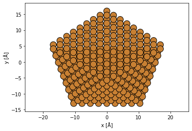
We create an atomic model of a decahedral copper nanoparticle. See our walkthough or our tutorial on atomic models.

cluster = Decahedron("Cu", 9, 2, 0)
cluster.rotate("x", -30)

abtem.show_atoms(cluster, plane="xy");

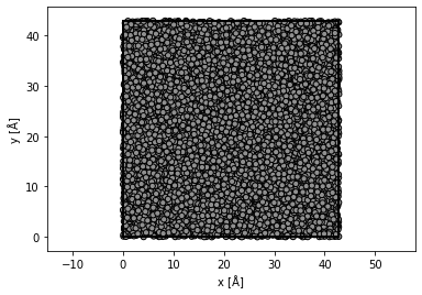
A rough model of amorphous carbon is created by randomly displacing the atoms of a diamond structure

substrate = ase.build.bulk("C", cubic=True)

# repeat diamond structure
substrate *= (12, 12, 10)

# displace atoms with a standard deviation of 50 % of the bond length
bondlength = 1.54  # Bond length
substrate.positions[:] += np.random.randn(len(substrate), 3) * 0.5 * bondlength

# wrap the atoms displaced outside the cell back into the cell
substrate.wrap()

abtem.show_atoms(substrate, plane="xy", merge=0.5);

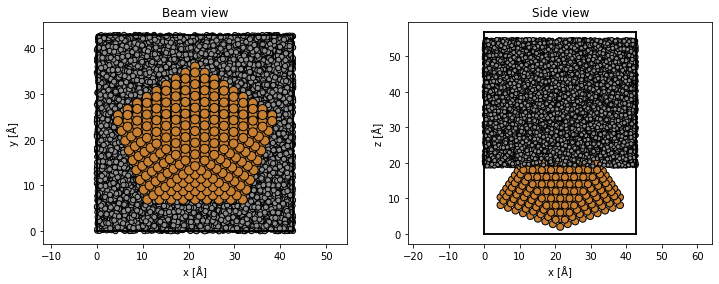
translated_cluster = cluster.copy()

translated_cluster.cell = substrate.cell
translated_cluster.center()
translated_cluster.translate((0, 0, -25))

atoms = substrate + translated_cluster

atoms.center(axis=2, vacuum=2)

fig, (ax1, ax2) = plt.subplots(1, 2, figsize=(12, 4))
abtem.show_atoms(atoms, plane="xy", ax=ax1, title="Beam view")
abtem.show_atoms(atoms, plane="xz", ax=ax2, title="Side view");

Potential

We create an ensemble of potentials using the frozen phonon model. See our walkthrough on frozen phonons.

frozen_phonons = abtem.FrozenPhonons(atoms, 4, sigmas=0.1)

We create a potential from the frozen phonons model, see walkthrough on potentials.

potential = abtem.Potential(
    frozen_phonons,
    gpts=1024,
    slice_thickness=2,
)

SMatrix

We create the ensemble of SMatrices by providing our potential, an acceleration voltage \(200 \ \mathrm{keV}\), a cutoff of the plane wave expansion of the probe of \(20 \ \mathrm{mrad}\) and an interpolation factor of 4 in both \(x\) and \(y\). See our tutorial on PRISM

s_matrix = abtem.SMatrix(
    potential=potential, energy=200e3, semiangle_cutoff=20, interpolation=4
)

s_matrix.shape

(4, 253, 1024, 1024)

Contrast transfer function

To include defocus, spherical aberration and other phase aberrations, we should define a contrast transfer function. Here we create one with a spherical aberration of \(20 \ \mu m\), the defocus is adjusted to the according Scherzer defocus.

Cs = 8e-6 * 1e10  # 20 micrometers

ctf = abtem.CTF(Cs=Cs, defocus="scherzer", energy=s_matrix.energy)

print(f"defocus = {ctf.defocus} Å")

defocus = 54.859099865741655 Å

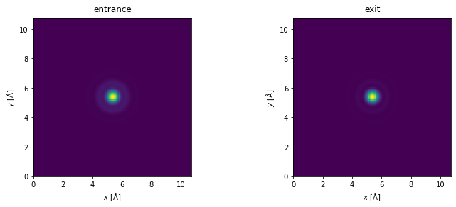
We always ensure that the interpolation factor is sufficiently small to avoid self-interaction errors. We can check that by showing the equivalent probe at the entrance and exit plane.

fig, (ax1, ax2) = plt.subplots(1, 2, figsize=(12, 4))
s_matrix.dummy_probes(plane="entrance", ctf=ctf).show(ax=ax1, title="entrance", power=1)
s_matrix.dummy_probes(plane="exit", ctf=ctf).show(ax=ax2, title="exit", power=1);

[########################################] | 100% Completed | 218.62 ms
[########################################] | 100% Completed | 108.73 ms

We should also check that our real space sampling is good enough for detecting electrons at our desired detector angles. In this case up to \(165 \ \mathrm{mrad}\). See our description of sampling.

s_matrix.cutoff_angles

(199.62780224577517, 199.62780224577517)

Create a CTF, a detector and a scan

detectors = abtem.FlexibleAnnularDetector()

flexible_measurement = s_matrix.scan(detectors=detectors, ctf=ctf)

flexible_measurement.compute()

[########################################] | 100% Completed | 20.05 s

<abtem.measurements.PolarMeasurements object at 0x000001DB9AD207F0>

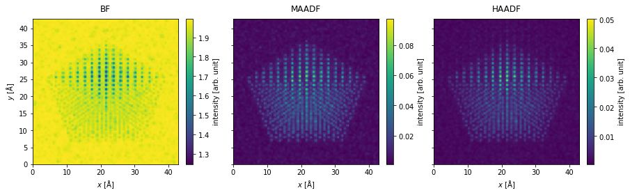
Integrate measurements

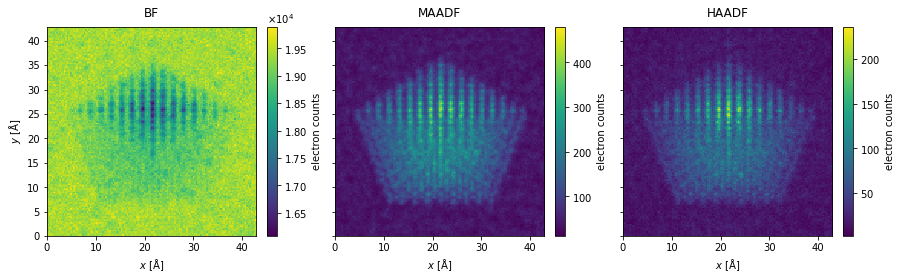
The measurements are integrated to obtain the bright field, medium-angle annular dark field and high-angle annular dark field signals.

bf_measurement = flexible_measurement.integrate_radial(0, s_matrix.semiangle_cutoff)
maadf_measurement = flexible_measurement.integrate_radial(45, 150)
haadf_measurement = flexible_measurement.integrate_radial(70, 190)

measurements = abtem.stack(
    [bf_measurement, maadf_measurement, haadf_measurement], ("BF", "MAADF", "HAADF")
)

measurements.show(
    explode=True,
    figsize=(14, 5),
    cbar=True,
);

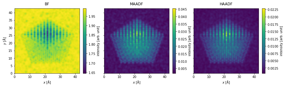
Postprocessing

filtered_measurements = measurements.gaussian_filter(0.35)

filtered_measurements.show(
    explode=True,
    figsize=(14, 5),
    cbar=True,
);

noisy_measurements = filtered_measurements.poisson_noise(dose_per_area=1e5)

noisy_measurements.show(
    explode=True,
    figsize=(14, 5),
    cbar=True,
);