import ase
import matplotlib.pyplot as plt
import numpy as np
from abtem.bloch import BlochWaves, StructureFactor

import abtem

abtem.config.set(
    {
        "precision": "float64",
        "device": "gpu",
    }
)
<abtem.core.config.set at 0x23bcdab9bd0>
Blochwave simulations#
Blochwave simulations, are implemented in abTEM, as an alternative to the multislice simulations, offering advantages under certain conditions. Blochwave allows for simulations of structures with arbitrary crystal rotations and arbitrary unit cells, which are difficult to handle in multislice due to the requirement of orthogonal and periodic unit cells. Blochwave is efficient for crystals described by small unit cells, but is scales as in both memory and time. Hence, becomes prohibitively expensive for large unit cells.
In this tutorial, we go through how to perform blochwave simulations as implemented in abTEM, and compare the simulation results to multislice.
Structure factor#
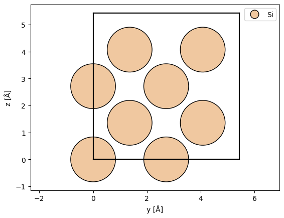
atoms = ase.build.bulk("Si", cubic=True)

abtem.show_atoms(atoms, legend=True, plane="yz")
(<Figure size 640x480 with 1 Axes>, <Axes: xlabel='y [Å]', ylabel='z [Å]'>)
k_max = 12

structure_factor = StructureFactor(
    atoms,
    k_max=k_max,
    parametrization="lobato",
)
sg_max = 0.1

bloch_waves = BlochWaves(
    structure_factor=structure_factor,
    energy=200e3,
    sg_max=sg_max,
)
len(bloch_waves)
3573
The selected beams can be accessed through the hkl property.
bloch_waves.hkl
array([[ 0,  0,  0],
       [ 0,  1,  0],
       [ 0,  2,  0],
       ...,
       [-1, -3,  0],
       [-1, -2,  0],
       [-1, -1,  0]])
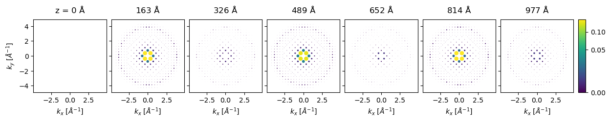
thicknesses = np.arange(0, 1086 + 0.1, 5.43)

diffraction_thickness_series = bloch_waves.calculate_diffraction_patterns(thicknesses)

diffraction_thickness_series
<abtem.measurements.IndexedDiffractionPatterns at 0x23bd3e78e50>
diffraction_thickness_series[::30].crop(k_max=4.5).block_direct().show(
    explode=True,
    scale=0.08,
    power=0.5,
    annotations=False,
    figsize=(14, 5),
    common_color_scale=True,
    cbar=True,
)
<abtem.visualize.visualizations.Visualization at 0x23bb0d06310>
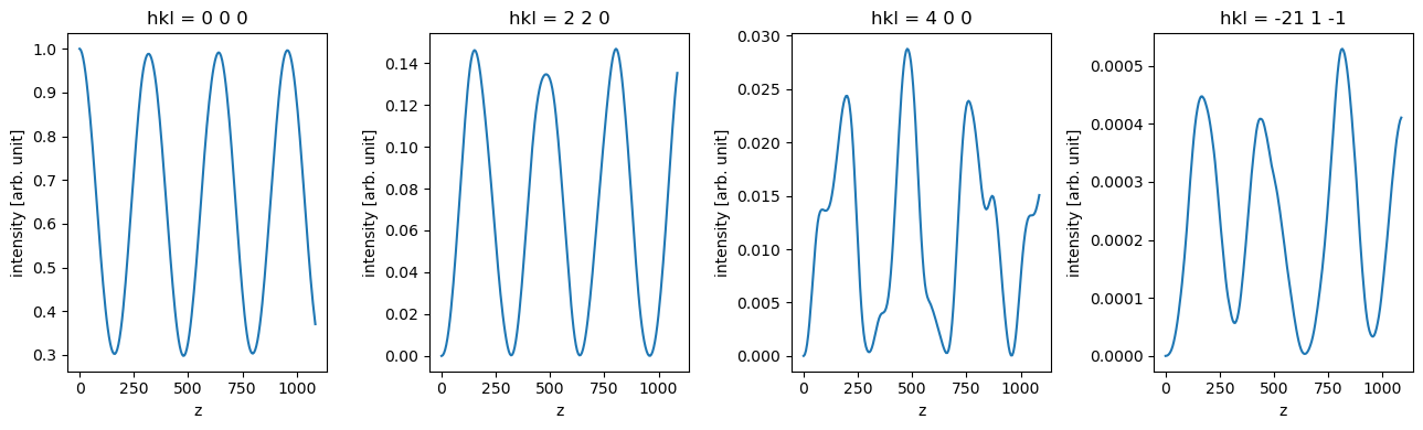
data_array = diffraction_thickness_series.to_data_array()
fig, axes = plt.subplots(1, 4, figsize=(13, 4))

for ax, hkl in zip(axes, ["0 0 0", "2 2 0", "4 0 0", "-21 1 -1"]):
    data_array.sel(hkl=hkl).plot(hue="hkl", ax=ax)

plt.tight_layout()
Rotations#
We can get diffraction intensities from other directions using the rotations method. Here, we rotate about \(z\) at \(4\) different angles between \(0\) and \(45 \ \mathrm{deg}\), for each \(z\) rotation we also rotate around \(x\) at \(5\) different angles between \(0\) and \(45 \ \mathrm{deg}\), i.e. resulting in \(16\) different simulations.
x = np.linspace(0, np.pi / 4, 4)
z = np.linspace(0, np.pi / 4, 4)

ensemble = bloch_waves.rotate("z", z, "x", x)

ensemble
<abtem.bloch.dynamical.BlochwaveEnsemble at 0x23c0b9cdbd0>
The previous operation produces a BlochwaveEmsenble object, we run the same calculate_diffraction_patterns method to create the tasks for running a Bloch wave simulation for each direction.
diffraction_patterns = ensemble.calculate_diffraction_patterns(thicknesses=1000)

diffraction_patterns.array
|
||||||||||||||||
diffraction_patterns.compute()
[########################################] | 100% Completed | 46.23 s
<abtem.measurements.IndexedDiffractionPatterns at 0x23c09c01cd0>
diffraction_patterns.shape
(4, 4, 32283)
diffraction_patterns = diffraction_patterns.remove_low_intensity(1e-6)
diffraction_patterns.crop(k_max=4).block_direct().show(
    explode=True,
    scale=0.03,
    power=0.5,
    annotation_kwargs={"threshold": 1},
    figsize=(14, 14),
)
<abtem.visualize.visualizations.Visualization at 0x23bd3ebc890>

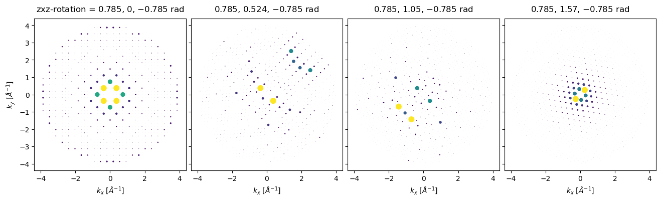
Arbitrary rotations may be given as a sequence of euler angles, for example, to rotate about a vector pointing along \((-1, 1, 0)\), we can rotate by \(\pi/4\) around \(z\), apply the desired rotations around \(x\), and then rotate back by \(-\pi/4\) around \(z\).
z = np.tile([np.pi / 4], (4,))
x = np.linspace(0, np.pi / 2, 4)

rotations = np.array([z, x, -z]).T
ensemble = bloch_waves.rotate("zxz", rotations)

diffraction_patterns = ensemble.calculate_diffraction_patterns(1000).compute()
[########################################] | 100% Completed | 9.69 ss
diffraction_patterns.crop(k_max=4).block_direct().show(
    explode=True,
    scale=0.03,
    power=0.5,
    annotation_kwargs={"threshold": 1},
    figsize=(14, 14),
)
<abtem.visualize.visualizations.Visualization at 0x23c7bc0f310>
Comparison to multislice#
k_max = 12

structure_factor = StructureFactor(
    atoms, k_max=k_max, parametrization="lobato", centering="F", thermal_sigma=0.078
)
potential_sf = structure_factor.get_projected_potential(slice_thickness=0.5)

potential_sf.sampling
(0.04082706766917293, 0.04082706766917293)
parametrization = abtem.parametrizations.LobatoParametrization(
    sigmas={"Si": 0.078 * np.sqrt(3)}
)

potential = (
    abtem.Potential(
        atoms,
        sampling=potential_sf.sampling,
        slice_thickness=0.1,
        projection="finite",
        parametrization=parametrization,
    )
    .build()
    .compute(progress_bar=False)
)
stack = abtem.stack(
    (potential.project(), potential_sf.project()), ("Direct", "From structure factor")
).compute()

stack.show(explode=True, common_color_scale=True, cbar=True);
[########################################] | 100% Completed | 205.39 ms

pw = abtem.PlaneWave(energy=200e3)

nz = int(1086 / potential.thickness)

repeated_potential = abtem.CrystalPotential(
    potential, repetitions=[1, 1, nz], exit_planes=potential.num_slices
)

exit_waves_ms = pw.multislice(potential=repeated_potential).compute()
[########################################] | 100% Completed | 14.37 s
bloch_waves = BlochWaves(
    structure_factor=structure_factor, energy=200e3, sg_max=sg_max, paraxial=True
)

len(bloch_waves)
901
exit_waves_bw = bloch_waves.calculate_exit_wave(
    repeated_potential.exit_thicknesses, gpts=exit_waves_ms.gpts
)
---------------------------------------------------------------------------
TypeError                                 Traceback (most recent call last)
Cell In[26], line 1
----> 1 exit_waves_bw = bloch_waves.calculate_exit_wave(
      2     repeated_potential.exit_thicknesses, gpts=exit_waves_ms.gpts
      3 )

TypeError: BlochWaves.calculate_exit_wave() missing 1 required positional argument: 'extent'
exit_waves_bw.shape
exit_waves_ms.shape
stack = abtem.stack(
    [exit_waves_bw, exit_waves_ms],
    axis_metadata={"label": "algorithm", "values": ["MS", "BW"]},
    axis=1,
)
stack.shape
stack[1::30].show(explode=True, figsize=(12, 4))
stacked_diffraction = (
    stack.to_cpu().diffraction_patterns().index_diffraction_spots(cell=atoms)
)
The difference below is mostly do to unconverged bloch wave.
data_array = stacked_diffraction.to_data_array()

fig, axes = plt.subplots(1, 4, figsize=(15, 4))

for ax, hkl in zip(axes, ["0 0 0", "2 2 0", "4 0 0", "-21 1 -1"]):
    data_array.sel(hkl=hkl).plot(hue="algorithm", ax=ax)

plt.tight_layout()
Rotating multislice simulations with periodic boundaries#
rotated_atoms = ase.build.bulk("Si", cubic=True)

angle = np.arctan(1 / 2)

rotated_atoms.rotate("x", angle * 180 / np.pi, rotate_cell=True)

rotated_atoms = abtem.orthogonalize_cell(rotated_atoms)

abtem.show_atoms(rotated_atoms, legend=True, plane="xy")
parametrization = abtem.parametrizations.LobatoParametrization(
    sigmas={"Si": 0.078 * np.sqrt(3)}
)

potential = abtem.Potential(
    atoms,
    sampling=0.05,
    slice_thickness=0.1,
    projection="finite",
    parametrization=parametrization,
)