Show code cell source Hide code cell source

import matplotlib.pyplot as plt
import numpy as np

import abtem

abtem.config.set({"local_diagnostics.progress_bar": False});

Wave functions

The multislice algorithm works by propagating the \(xy\) part of the wave function (defined as \(\psi\) in the appendix) through the electrostatic potential. To start the propagation, we need to assume the initial conditions for the wave function, i.e. a wave function describing the electron beam formed by the electron optics before the sample.

abTEM defines three types of wave functions:

• PlaneWave: Simulate HRTEM, SAED or other imaging modes with parallel-beam plane wave illumination.

• Probe: Simulate CBED, STEM or other imaging modes with a converged electron beam.

• Waves: Defines any custom wave function. PlaneWave and Probe can be converted to Waves.

See also

abTEM implments the PRISM algorithm using the SMatrix, which is not included in the list above. However, in most ways it can be used similar to Probe; see our tutorial on PRISM in abTEM.

Plane wave functions

The default plane wave is just defined to be equal to unity everywhere in the plane

\[ \psi(\vec{r}) = 1 \quad , \]

where \(\vec{r} = (x, y)\) is the real space coordinate in the \(x\)- and \(y\)-direction. While mathematically, those coordinates are usually considered to be continuous, in a numerical simulation we have define a discrete grid with a finite extent to represent them.

We create a plane wave on a \(256 \times 256\) grid with a lateral extent of \(5\times 5\) \(\mathrm{Å}^2\) and an energy of \(300 \ \mathrm{keV}\).

plane_wave = abtem.PlaneWave(gpts=256, extent=5, energy=300e3)

The real-space sampling, or pixel size, is calculated by dividing the extent by the number of grid points (gpts). The properties related to the grid, i.e. the extent, gpts and sampling, can be accessed as properties of the PlaneWave object.

plane_wave.extent, plane_wave.gpts, plane_wave.sampling

((5.0, 5.0), (256, 256), (0.01953125, 0.01953125))

The grid is fully defined from just two of the three quantities listed above, and thus we may pick any combination of two to define it.

The relativistic wavelength of the electron beam may be accessed as:

print(f"Wavelength: {plane_wave.wavelength:.4f} Å")

Wavelength: 0.0197 Å

Note

abTEM uses the same unit conventions as ASE, as defined in the ase.units module. Thus, electron volts (eV), Ångström (Å), and atomic mass units are defined as 1.0. The electrostatic potential is given in (eV / e). Angles in abTEM are for convenience given in milliradians (mrad).

We can turn the PlaneWave into a generic Waves by using build.

waves = plane_wave.build()

The Waves describe the wave function as a complex Dask array (see our page on parallelization), as accessed below.

waves.array

Array Chunk Bytes 512.00 kiB 512.00 kiB Shape (256, 256) (256, 256) Dask graph 1 chunks in 2 graph layers Data type complex64 numpy.ndarray

After computing the values of the wave function, it will be described as a NumPy array.

waves.compute()

waves.array

array([[1.+0.j, 1.+0.j, 1.+0.j, ..., 1.+0.j, 1.+0.j, 1.+0.j],
       [1.+0.j, 1.+0.j, 1.+0.j, ..., 1.+0.j, 1.+0.j, 1.+0.j],
       [1.+0.j, 1.+0.j, 1.+0.j, ..., 1.+0.j, 1.+0.j, 1.+0.j],
       ...,
       [1.+0.j, 1.+0.j, 1.+0.j, ..., 1.+0.j, 1.+0.j, 1.+0.j],
       [1.+0.j, 1.+0.j, 1.+0.j, ..., 1.+0.j, 1.+0.j, 1.+0.j],
       [1.+0.j, 1.+0.j, 1.+0.j, ..., 1.+0.j, 1.+0.j, 1.+0.j]],
      dtype=complex64)

The normalization of the wave function used above ensures that the intensity per area is constant when the grid is changed. However, this is not a very natural normalization in reciprocal space, and we may instead define the plane wave such that the total intensity of the plane wave is, i.e. the wave function (in reciprocal space) is given by

\[ \hat{\psi}(\vec{k}) = \delta(0) \quad . \]

We create a plane wave with this normalization by setting normalize=True.

normalized_plane_wave = abtem.PlaneWave(
    gpts=256, extent=5, energy=300e3, normalize=True
)

Probe wave functions

In abTEM, a focused beam of electrons, or Probe, is defined in Fourier space as

\[ \hat{\psi}(\vec{k}) = A(\vec{k}) \ \exp(-i \chi(\vec{k})) \quad , \]

where \(A(k)\) is the aperture function, \(\chi(\vec{k})\) is the phase error and \(\vec{k} = (k_x, k_y)\) is the spatial frequency in \(x\) and \(y\), respectively. The real-space probe is just the inverse Fourier transform

\[ \psi(\vec{r}) = \mathcal{F}^{-1} \left[ \hat{\psi}(\vec{k}) \right] \quad . \]

The probe wave function is normalized such that its intensity sums to \(1\) in Fourier space

\[ \int \|\hat{\psi}\|^2 d\vec{k} = 1 \quad . \]

We create a probe with a sampling of \(0.05 \ \mathrm{Å}\), an extent of \(20\times 20\) \(\mathrm{Å}^2\), an energy of \(80 \ \mathrm{keV}\), a convergence semiangle (semiangle_cutoff) of \(30 \ \mathrm{mrad}\), a defocus (C10; note the common negative sign convention here) of \(-50 \ \mathrm{Å}\) and spherical aberration (Cs) of \(-50 \ \mathrm{\mu m}\) (note the conversion to \(\mathrm{m}\) and then to \(\mathrm{Å}\)).

probe = abtem.Probe(
    sampling=0.05,
    extent=20,
    energy=80e3,
    semiangle_cutoff=20,
    C10=50,
    Cs=-50e-6 * 1e10,
)

See also

See our introduction to the contrast transfer function for a full list of phase aberrations.

We can again turn the Probe into the generic Waves by using build, which, as the plane wave, is represented by a Dask array.

waves = probe.build()

waves.array

Array Chunk Bytes 1.22 MiB 1.22 MiB Shape (400, 400) (400, 400) Dask graph 1 chunks in 4 graph layers Data type complex64 numpy.ndarray

Visualizing the wave function

To visualize the wave function using abTEM’s built-in visualization module, we first have to convert it to a measurement type. The most common methods are intensity and diffraction_patterns, which will return a measurement of type Images and DiffractionPatterns, respectively.

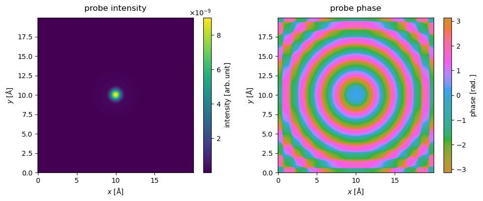
The real space intensity, \(\|\psi\|^2\), and phase of the probe is calculated and shown below. The parameter cbar=True displays the color intensity scale.

intensity = probe.build().intensity().compute()
phase = probe.build().phase()

fig, (ax1, ax2) = plt.subplots(1, 2, figsize=(10,4))

intensity.show(cbar=True, title="probe intensity", ax=ax1)
phase.show(cbar=True, title="probe phase", cmap="hsluv", ax=ax2)

plt.tight_layout()

Note

The axes convention in abTEM for arrays representing a wave functions assigns the first axis to the \(x\)-axis and the second axis to the \(y\)-axis. This is different from the convention often used for images, and the convention used by matplotlib. The correct way of displaying an array representing the wave function intensity from abTEM with matplotplib is given below.

import matplotlib.pyplot as plt
image = waves.intensity().array
plt.imshow(image.T, extent=[0, waves.extent[0], 0, waves.extent[1]], origin="lower")

The image is transposed to reverse the order of the axes and the direction of the \(y\)-axis is reversed by setting origin="lower".

Showing a lineprofile sometimes provides a more readily understable visualization. We use interpolate_line_at_position to create a LineProfile across the center of the probe intensity.

lineprofile = intensity.interpolate_line_at_position(
    center=(10, 10), angle=0, extent=10
)

lineprofile.show()

<abtem.visualize.visualizations.Visualization at 0x1a346901010>

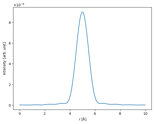
It is often useful to know the width of the probe. Below we calculate the width at \(0.5\) of the height of the probe (i.e. the full width at half-maximum, FWHM).

fwhm = lineprofile.width(height=0.5)

print(f"FWHM = {fwhm.item():.2f} Å")

FWHM = 1.11 Å

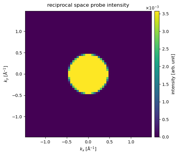
The Fourier-space intensity, \(\|\hat{\psi}\|^2\), is calculated and shown below. We set max_angle=60 to only include angles up to \(60 \ \mathrm{mrad}\).

diffraction_patterns = probe.build().diffraction_patterns(max_angle=60)

visualization = diffraction_patterns.show(
    cbar=True, title="reciprocal space probe intensity"
)

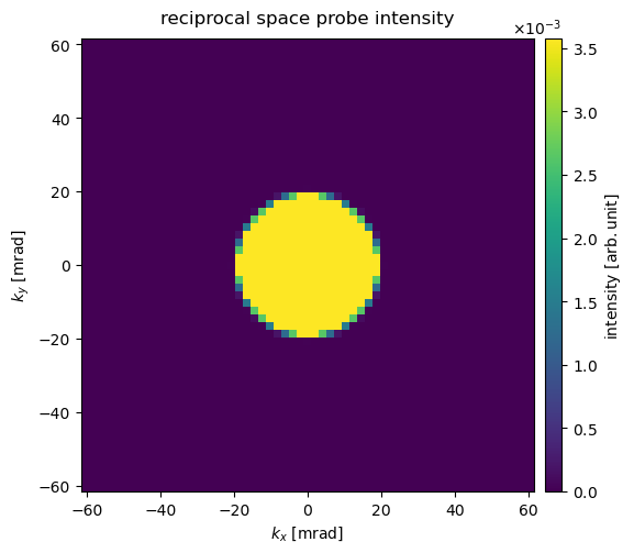
Alternative to reciprocal-space units, we can display diffraction patterns in angular units by using the keyword units='mrad'.

visualization = diffraction_patterns.show(
    cbar=True, units="mrad", title="reciprocal space probe intensity"
)

Wave-function ensembles

In general, Waves can represent an ensemble of wave functions as a multidimensional array. The last two dimensions of Waves represent the spatial dimensions, which are the mandatory or base dimensions of the object. Any preceeding dimension is an optional ensemble dimension. The ensemble dimensions may represent a range of defocii, positions, frozen phonons, tilt and more. In computations, abTEM will automatically parallelize over the ensemble dimensions.

As an example, we create an ensemble of probes with different values for their defocus.

defocus_series = np.linspace(0, 100, 5)

probe_focal_series = abtem.Probe(
    gpts=256,
    extent=25,
    energy=80e3,
    semiangle_cutoff=30,
    defocus=defocus_series,
)

waves_focal_series = probe_focal_series.build().compute()

Warning

Not every parameter in abTEM allows setting with an array, check the API documentation for arguments admitting BaseDistribution as a value.

Now Waves is a 1D ensemble of 2D wave functions, hence its shape is 3D.

waves_focal_series.shape

(5, 256, 256)

We can inspect the axes_metadata property to see that the first axis is the ensemble ParameterAxis over C10, equivalent to negative defocus, and the base are RealSpaceAxis.

waves_focal_series.axes_metadata

type           label    coordinates
-------------  -------  ------------------------
ParameterAxis  C10 [Å]  -0.00 -25.00 ... -100.00
RealSpaceAxis  x [Å]    0.00 0.10 ... 24.90
RealSpaceAxis  y [Å]    0.00 0.10 ... 24.90

We can obtain an ensemble of Images, which can be conveniently shown in an “exploded” plot.

waves_focal_series.show(explode=True, figsize=(14, 3));

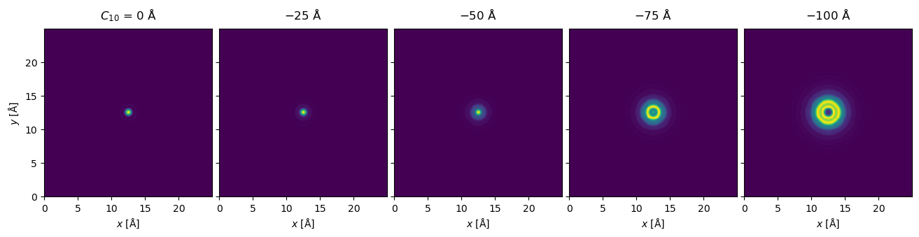
The plot above scales the maximum intensity of each panel. You can set common_color_scale=True to get a better representation of the relative intensity between each panel.

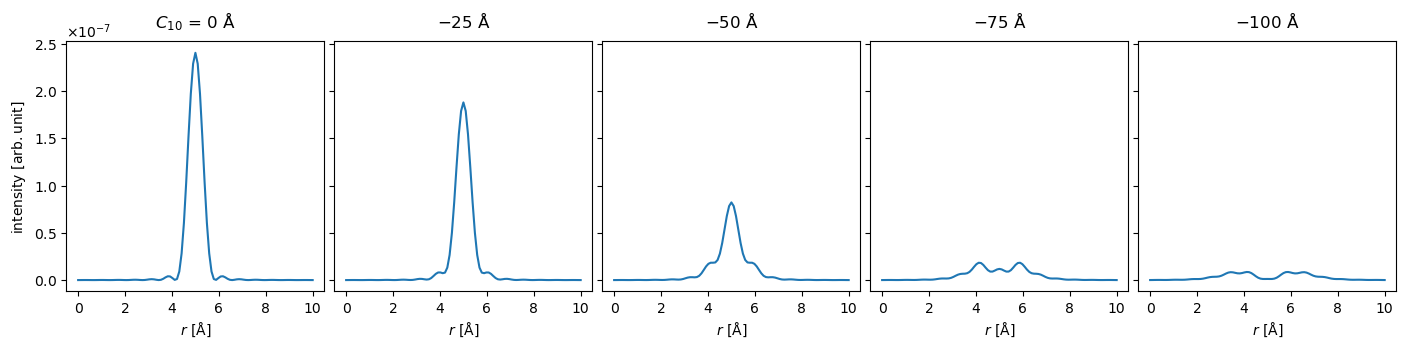
Alternatively, we can show a selection of lineprofiles. When using methods, such as interpolate_line_profiles, on an ensemble, it will be applied to each member of the ensemble. The show method handles these automatically.

line_profiles = waves_focal_series.intensity().interpolate_line_at_position(
    center=(12.5, 12.5), angle=0, extent=10
)

visualization = line_profiles.show(explode=True, figsize=(15, 3), common_scale=True);

Waves can have any number of ensemble dimensions, for example, we can add two additional axes representing a scan in the \(x\)- and \(y\)- direction, thus producing a 3D ensemble of 2D wave functions.

scan = abtem.GridScan()

waves_focal_series_scanned = probe_focal_series.build(scan=scan)

waves_focal_series_scanned.array

Array Chunk Bytes 13.01 GiB 105.00 MiB Shape (5, 73, 73, 256, 256) (5, 7, 6, 256, 256) Dask graph 143 chunks in 5 graph layers Data type complex64 numpy.ndarray

Be careful about running the compute method after adding ensemble dimensions before applying a reduction operation, such as taking an ensemble mean or applying a detector. The above ensemble would take \(\sim 13 \ \mathrm{GB}\) of memory.